“He was how old??”
Analysing historical data about Members of Parliament
Two weeks ago, a friend sent along the Wikipedia page of Ivan Grose. Ivan Grose robbed a bank when he was 29. Notable as that is, the fact that caught my eye was that he was then elected as a Member of Parliament (MP)—36 years later, at the age of 65.
65 seemed to me rather up there for an age at first election. This got me wondering: how old are MPs usually when they’re first elected?
Some quick poking around Google yielded few results, so I decided to take the opportunity to practice my data analysis skills. I figured I could find a dataset of Canadian MPs and then analyze it to answer my own question.
Finding such a dataset took a bit of work. The House of Commons publishes open data about current MPs, but not MPs from previous Parliaments. The Linked Parliamentary Data Project (LiPaD) offers a dataset on politicians, including those from previous Parliaments. The dataset is in XML format, which requires more effort to load and analyze than a simple CSV file. I noted the LiPaD dataset as a viable option, but kept looking.
Finally, I found the Library of Parliament’s parliamentarians search interface. At first glance this seemed only useful for searching, but two features make it useful for our purposes: searching without any filters returns every record in the dataset (i.e. every parliamentarian); there’s an export button to download search results in the easy-to-use CSV format. These two features combined allow us to download a CSV containing the information of every Canadian parliamentarian (or, in this case, every MP). I noted my instructions for extracting the data from this “API by accident” in GitHub.
With the CSV in hand, I then did some basic analysis with R and the tidyverse packages. You can see the code in my GitHub repo.
I first read the CSV and renamed the columns:
import_lop_mps <- read_csv("data/lop-mps.csv") %>%
  rename(
    picture = Picture,
    name = Name,
    birth_date = `Date of Birth`,
    birth_city = `City of Birth`,
    birth_province_region = `Province/Region of Birth`,
    birth_country = `Country of Birth`,
    deceased_date = `Deceased Date`,
    gender = Gender,
    profession = Profession,
    seat_riding_senatorial_division = `Riding/Senatorial Division`,
    seat_province_territory = `Province/Territory`,
    political_affiliation = `Political Affiliation`,
    date_of_parliamentary_entry = `Date Appointed/Date of First Election`,
    role_type_of_parliamentarian = `Type of Parliamentarian`,
    role_minister = Minister,
    role_critic = Critic,
    years_of_service = `Years of Service`,
    military_service = `Military Service`
  )
I then approximated the age of election, creating a smaller working table (with just the MP’s name, party, birth date, date of entry to Parliament, their age when first entering Parliament, and their years of service):
age_at_election <- import_lop_mps %>%
  filter(birth_date != "") %>%
  mutate(age_at_first_election = as.integer(substr(as.character(date_of_parliamentary_entry), 1, 4)) - as.integer(substr(birth_date, 1, 4))) %>%
  mutate(years_of_service = as.numeric(str_extract(years_of_service, "(\\d+)")) / 365) %>%
  select(name, birth_date, political_affiliation, date_of_parliamentary_entry, age_at_first_election, years_of_service) %>%
  arrange(age_at_first_election)
I then generated some summary statistics about the age of first election:
age_at_election %>%
  summarize(
    mean_age_at_first_election = mean(age_at_first_election, na.rm = TRUE),
    median_age_at_first_election = median(age_at_first_election, na.rm = TRUE),
    min_age_at_first_election = min(age_at_first_election, na.rm = TRUE),
    max_age_at_first_election = max(age_at_first_election, na.rm = TRUE)
  )
This yields the following values:
| Key | Value |
|---|---|
| Mean | 45.5 |
| Median | 45 |
| Minimum | 20 |
| Maximum | 76 |
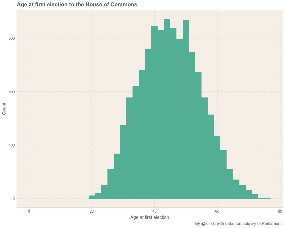
I also generated a histogram of the data:
age_at_election %>%
  ggplot(aes(x = age_at_first_election)) +
  geom_histogram(binwidth = 2) +
  scale_x_continuous(limits = c(0, NA)) +
  labs(
    title = "Age at first election to the House of Commons",
    x = "Age at first election",
    y = "Count",
    caption = "By @lchski with data from Library of Parliament."
  )
Finally, to put the election of Ivan Grose into context, I calculated the percentage of MPs first elected at age 65 or older:
(age_at_election %>% filter(age_at_first_election >= 65) %>% count() %>% pull(n)) / (age_at_election %>% count() %>% pull(n))
This works out to 2.51%. Grose is definitely in the minority in this case!
Hopefully this offers a useful overview of how to go from having a question to finding an answer to it with data. If you’re interested in using structured data to answer historical questions, check out Ian Milligan’s article, “Open Data’s Potential for Political History”.